3DCNN 实践-视频行为识别

本教程使用 TensorFlow 搭建一个 3D 卷积神经网络，模型采用 (2+1)D 卷积（空间卷积 + 时间卷积分离）和残差连接，在 Kaggle 人体动作识别视频数据集上进行训练。实现对视频中的人物行为进行分类。

1. 环境准备
#

1.1 检查 GPU
#

!nvidia-smi

1.2 安装依赖
#

!pip install remotezip einops
!pip install -q git+https://github.com/tensorflow/docs

1.3 导入库
#

import tensorflow as tf
import cv2
import numpy as np
import remotezip as rz
import os
import tqdm
import random
import pathlib
import itertools
import collections
import imageio
from IPython import display
from urllib import request
from tensorflow_docs.vis import embed
import keras
from keras import layers
import matplotlib.pyplot as plt
import einops
import seaborn as sns

2. 数据集下载与探索
#

2.1 下载视频数据集
#

从 Kaggle 下载人体动作识别视频数据集，包含 7 类行为：

URL = 'https://www.kaggle.com/api/v1/datasets/download/sharjeelmazhar/human-activity-recognition-video-dataset?datasetVersionNumber=1'

video_format = 'mp4'

2.2 列出 ZIP 内的文件
#

def list_files_from_zip_url(zip_url):
  files = []
  with rz.RemoteZip(zip_url) as zip:
    for zip_info in zip.infolist():
      files.append(zip_info.filename)
  return files

files = list_files_from_zip_url(URL)
files = [f for f in files if f.endswith(f'.{video_format}')]
files[:10]

2.3 提取类别名称
#

def get_class(fname):
  return fname.split('/')[1]

get_class(files[0])

'Clapping'

2.4 统计各类别样本量
#

def get_files_for_class(files):
  files_for_class = collections.defaultdict(list)
  for fname in files:
    class_name = get_class(fname)
    files_for_class[class_name].append(fname)
  return files_for_class

files_for_class = get_files_for_class(files)
classes = list(files_for_class.keys())

for i in range(len(classes)):
  class_name = classes[i]
  files_num = len(files_for_class[class_name])
  print(i, class_name, files_num)

类别	样本数
Clapping	146
Meet and Split	147
Sitting	156
Standing Still	174
Walking While Reading Book	176
Walking While Using Phone	143
Walking	171

3. 数据划分与下载
#

3.1 类别子集选择
#

选择前 7 类，每类取 50 个视频：

def select_subset_of_classes(files_for_class, classes, num_per_class):
  files_subset = dict()
  for class_name in classes:
    class_files = files_for_class[class_name]
    files_subset[class_name] = class_files[:num_per_class]
  return files_subset

NUM_CLASS = 7
NUM_PER_CLASS = 50

files_subset = select_subset_of_classes(files_for_class, classes[:NUM_CLASS], NUM_PER_CLASS)
list(files_subset.keys())

3.2 从 ZIP 下载文件
#

def download_from_zip(zip_url, to_dir, file_names):
  with rz.RemoteZip(zip_url) as zip:
    for fn in tqdm.tqdm(file_names):
      class_name = get_class(fn)
      zip.extract(fn, str(to_dir / class_name))
      unzipped_file = to_dir / class_name / fn
      fn = pathlib.Path(fn).parts[-1]
      output_file = to_dir / class_name / fn
      unzipped_file.rename(output_file)

3.3 数据划分函数
#

def split_class_lists(files_for_class, count):
  split_files = []
  remain = {}
  for class_name in files_for_class:
    split_files.extend(files_for_class[class_name][:count])
    remain[class_name] = files_for_class[class_name][count:]
  return split_files, remain

def download_and_split_files(zip_url, num_classes, splits, to_dir):
  files = list_files_from_zip_url(zip_url)
  for f in files:
    path = os.path.normpath(f)
    tokens = path.split(os.sep)
    if len(tokens) <= 2:
      files.remove(f)

  files_for_class = get_files_for_class(files)
  classes = list(files_for_class.keys())[:num_classes]

  for class_name in classes:
    random.shuffle(files_for_class[class_name])

  files_for_class = {x: files_for_class[x] for x in classes}

  dirs = {}
  for split_name, split_count in splits.items():
    print(split_name, ":")
    split_dir = to_dir / split_name
    split_files, files_for_class = split_class_lists(files_for_class, split_count)
    download_from_zip(zip_url, split_dir, split_files)
    dirs[split_name] = split_dir

  return dirs

3.4 执行划分与下载
#

每类取 30 个训练、10 个验证、10 个测试：

to_dir = pathlib.Path('./dataset')
subset_paths = download_and_split_files(URL, NUM_CLASS, {"train": 30, "val": 10, "test": 10}, to_dir)

train : 100%| 210/210 [16:41, 4.77s/it]
val : 100%| 70/70 [04:59, 4.27s/it]
test : 100%| 70/70 [05:09, 4.42s/it]

3.5 验证数据分布
#

train_count = len(list(to_dir.glob(f'train/*/*.{video_format}')))
val_count = len(list(to_dir.glob(f'val/*/*.{video_format}')))
test_count = len(list(to_dir.glob(f'test/*/*.{video_format}')))
print('train: ', train_count)
print('val: ', val_count)
print('test: ', test_count)
print('total: ', total)

train:  210
val:  70
test:  70
total:  350

每类验证集分布：

Clapping: 10
Standing Still: 10
Meet and Split: 10
Sitting: 10
Walking: 10
Walking While Reading Book: 10
Walking While Using Phone: 10

共 350 个视频，每个类别 30 训练 + 10 验证 + 10 测试。

四、视频帧提取与预处理
#

视频数据不能像图片那样直接输入神经网络，核心挑战在于：

视频长度不固定
需要同时保留空间信息（画面内容）和时序信息（动作变化）
需对帧进行标准化处理

单帧格式化
#

def format_frame(frame, output_size):
  frame = tf.image.convert_image_dtype(frame, tf.float32)
  frame = tf.image.resize_with_pad(frame, *output_size)
  return frame

将单帧转换为 float32，并缩放到统一尺寸（224×224），保持宽高比填充（resize_with_pad）。

从视频文件中提取帧序列
#

def frames_from_video_file(video_path, n_frames, output_size = (224, 224), frame_step = 15):
  result = []
  src = cv2.VideoCapture(str(video_path))

  video_length = src.get(cv2.CAP_PROP_FRAME_COUNT)
  need_length = 1 + (n_frames - 1) * frame_step

  if need_length > video_length:
    start = 0
  else:
    max_start = video_length - need_length
    start = random.randint(0, max_start + 1)

  src.set(cv2.CAP_PROP_POS_FRAMES, start)
  ret, frame = src.read()
  result.append(format_frame(frame, output_size))

  for _ in range(n_frames - 1):
    for _ in range(frame_step):
      ret, frame = src.read()
    if ret:
      frame = format_frame(frame, output_size)
      result.append(frame)
    else:
      result.append(np.zeros_like(result[0]))
  src.release()
  result = np.array(result)[..., [2, 1, 0]]

  return result

关键设计：

frame_step=15：跳帧采样，每 15 帧取一帧，避免连续帧信息冗余
随机起始位置：如果视频足够长，从随机位置开始采样，增强数据多样性
不足补零：视频不够长时，用零填充（np.zeros_like）
BGR→RGB：[..., [2, 1, 0]] 将 OpenCV 的 BGR 转为 RGB

帧生成器类
#

class FrameGenerator:
  def __init__(self, path, n_frames, training = False):
    self.path = path
    self.n_frames = n_frames
    self.training = training
    self.class_names = sorted(set(p.name for p in self.path.iterdir() if p.is_dir()))
    self.class_ids_for_name = dict((name, idx) for idx, name in enumerate(self.class_names))

  def get_files_and_class_names(self):
    video_paths = list(self.path.glob(f'*/*.{video_format}'))
    classes = [p.parent.name for p in video_paths]
    return video_paths, classes

  def __call__(self):
    video_paths, classes = self.get_files_and_class_names()
    pairs = list(zip(video_paths, classes))

    if self.training:
      random.shuffle(pairs)

    for path, name in pairs:
      video_frames = frames_from_video_file(path, self.n_frames)
      label = self.class_ids_for_name[name]
      yield video_frames, label

FrameGenerator 封装了完整的帧提取流程：

遍历数据集目录下的所有视频文件
对每个视频调用 frames_from_video_file 提取帧序列
训练时打乱顺序（shuffle），验证/测试时保持顺序
每帧形状：(10, 224, 224, 3)（10 帧 × 224×224 × RGB）

五、数据管道构建
#

使用 tf.data.Dataset 构建高效的数据流水线。

output_signature = (
    tf.TensorSpec(shape = (None, None, None, 3), dtype = tf.float32),
    tf.TensorSpec(shape = (), dtype = tf.int16)
)

train_ds_ = tf.data.Dataset.from_generator(
    FrameGenerator(subset_paths['train'], 10, training=True),
    output_signature = output_signature
)

val_ds_ = tf.data.Dataset.from_generator(
    FrameGenerator(subset_paths['val'], 10),
    output_signature = output_signature
)

test_ds_ = tf.data.Dataset.from_generator(
    FrameGenerator(subset_paths['test'], 10),
    output_signature = output_signature
)

AUTOTUNE = tf.data.AUTOTUNE
batch_size = 8

train_ds = train_ds_.cache().shuffle(1000).prefetch(buffer_size = AUTOTUNE).batch(batch_size)
val_ds = val_ds_.cache().shuffle(1000).prefetch(buffer_size = AUTOTUNE).batch(batch_size)
test_ds = test_ds_.cache().shuffle(1000).prefetch(buffer_size = AUTOTUNE).batch(batch_size)

output_signature：指定生成器输出的张量类型和形状，None 维度表示帧数、高、宽可变
cache()：将数据集缓存到内存，加速后续 epoch 的读取
shuffle(1000)：随机打乱样本顺序
prefetch(AUTOTUNE)：在 GPU 训练的同时预加载下一批数据，隐藏 I/O 延迟
batch(8)：每批 8 个视频（每个视频 10 帧）

批次形状：(8, 10, 224, 224, 3) — 8 个视频 × 10 帧 × 224 × 224 × RGB

六、(2+1)D 卷积模型
#

本教程的核心创新是将 3D 卷积分解为空间卷积 + 时间卷积，称为 Conv2Plus1D。

Conv2Plus1D：分解 3D 卷积
#

class Conv2Plus1D(keras.layers.Layer):
  def __init__(self, filters, kernel_size, padding):
    super().__init__()
    self.seq = keras.Sequential([
        # Spatial decomposition
        layers.Conv3D(
            filters = filters,
            kernel_size = (1, kernel_size[1], kernel_size[2]),
            padding = padding
        ),
        # Temporal decomposition
        layers.Conv3D(
            filters = filters,
            kernel_size = (kernel_size[0], 1, 1),
            padding = padding
        )
    ])

  def call(self, x):
    return self.seq(x)

为什么分解？一个 (3, 3, 3) 的 3D 卷积核有 27 个参数/位置，而分解为 (1, 3, 3) 空间部分（9 个位置）+ (3, 1, 1) 时间部分（3 个位置），总共 12 个位置，参数量减少 55%。

这种分解：

降低过拟合风险
加速训练
在视频任务上通常表现不逊于完整 3D 卷积

残差模块
#

class ResidualMain(keras.layers.Layer):
  def __init__(self, filters, kernel_size):
    super().__init__()
    self.seq = keras.Sequential([
        Conv2Plus1D(
            filters = filters,
            kernel_size = kernel_size,
            padding = 'same'
        ),
        layers.LayerNormalization(),
        layers.ReLU(),
        Conv2Plus1D(
            filters = filters,
            kernel_size = kernel_size,
            padding = 'same'
        ),
        layers.LayerNormalization(),
    ])

  def call(self, x):
    return self.seq(x)

残差结构：两个 Conv2Plus1D + LayerNorm + ReLU，通过跳跃连接让梯度直接流通。

class Project(keras.layers.Layer):
  def __init__(self, units):
    super().__init__()
    self.seq = keras.Sequential([
        layers.Dense(units),
        layers.LayerNormalization(),
    ])

  def call(self, x):
    return self.seq(x)

def add_residual_block(input, filters, kernel_size):
  out = ResidualMain(filters, kernel_size)(input)
  res = input

  if out.shape[-1] != input.shape[-1]:
    res = Project(out.shape[-1])(res)

  return layers.add([res, out])

当残差路径的通道数发生变化时，Project 层通过 Dense 将跳跃连接投影到相同维度。

视频下采样
#

class ResizeVideo(keras.layers.Layer):
  def __init__(self, height, width):
    super().__init__()
    self.height = height
    self.width = width
    self.resizing_layer = layers.Resizing(self.height, self.width)

  def call(self, video):
    old_shape = einops.parse_shape(video, 'b t h w c')
    images = einops.rearrange(video, 'b t h w c -> (b t) h w c')
    images = self.resizing_layer(images)
    videos = einops.rearrange(
        images, '(b t) h w c -> b t h w c',
        t = old_shape['t'])
    return videos

使用 einops 在批次-时间维度间重排，将视频帧展开为独立图片进行下采样，再恢复为视频张量。

完整模型结构
#

input_shape = (None, 10, HEIGHT, WIDTH, 3)
input = layers.Input(shape = (input_shape[1:]))
x = input

x = Conv2Plus1D(filters = 16, kernel_size = (3, 7, 7), padding = 'same')(x)
x = layers.BatchNormalization()(x)
x = layers.ReLU()(x)
x = ResizeVideo(HEIGHT // 2, WIDTH // 2)(x)

# Block 1
x = add_residual_block(x, 16, (3, 3, 3))
x = ResizeVideo(HEIGHT // 4, WIDTH // 4)(x)

# Block 2
x = add_residual_block(x, 32, (3, 3, 3))
x = ResizeVideo(HEIGHT // 8, WIDTH // 8)(x)

# Block 3
x = add_residual_block(x, 64, (3, 3, 3))
x = ResizeVideo(HEIGHT // 16, WIDTH // 16)(x)

# Block 4
x = add_residual_block(x, 128, (3, 3, 3))

x = layers.GlobalAveragePooling3D()(x)
x = layers.Flatten()(x)
x = layers.Dense(10)(x)

model = keras.Model(input, x)

frames, label = next(iter(train_ds))
model.build(frames)

keras.utils.plot_model(model, expand_nested=True, dpi=60, show_shapes=True)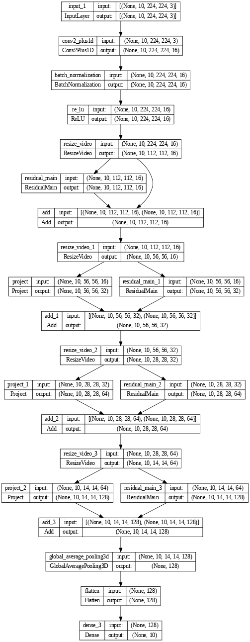

架构总览：

层级	组件	输出空间尺寸	通道数
输入	—	224×224	3
Stem	Conv2Plus1D(3,7,7) + BN + ReLU	224×224	16
Down 1	ResizeVideo /2	112×112	16
Block 1	Residual(3,3,3)	112×112	16
Down 2	ResizeVideo /2	56×56	16
Block 2	Residual(3,3,3)	56×56	32
Down 3	ResizeVideo /2	28×28	32
Block 3	Residual(3,3,3)	28×28	64
Down 4	ResizeVideo /2	14×14	64
Block 4	Residual(3,3,3)	14×14	128
Head	GAP + Flatten + Dense(10)	—	10

空间维度从 224 逐级下采样到 14，通道数从 3 扩展到 128，最终通过全局平均池化和全连接层输出 10 类 logits。

七、模型编译与训练
#

model.compile(
    loss = keras.losses.SparseCategoricalCrossentropy(from_logits=True),
    optimizer = keras.optimizers.Adam(learning_rate=0.0001),
    metrics = ['accuracy']
)

损失函数：SparseCategoricalCrossentropy（标签为整数，非 one-hot）
优化器：Adam，学习率 0.0001（较小，适合视频任务的稳定性）
评估指标：准确率

history = model.fit(
    x = train_ds,
    epochs = 50,
    validation_data = val_ds
)

....
Epoch 45/50
27/27 [==============================] - 4s 161ms/step - loss: 0.6367 - accuracy: 0.7667 - val_loss: 1.1064 - val_accuracy: 0.6143
Epoch 46/50
27/27 [==============================] - 4s 160ms/step - loss: 0.6492 - accuracy: 0.7619 - val_loss: 1.1573 - val_accuracy: 0.6286
Epoch 47/50
27/27 [==============================] - 4s 159ms/step - loss: 0.6652 - accuracy: 0.7476 - val_loss: 1.2028 - val_accuracy: 0.5143
Epoch 48/50
27/27 [==============================] - 4s 160ms/step - loss: 0.7080 - accuracy: 0.7286 - val_loss: 1.0872 - val_accuracy: 0.5857
Epoch 49/50
27/27 [==============================] - 4s 161ms/step - loss: 0.5570 - accuracy: 0.8381 - val_loss: 1.1155 - val_accuracy: 0.6000
Epoch 50/50
27/27 [==============================] - 4s 160ms/step - loss: 0.6262 - accuracy: 0.7857 - val_loss: 0.9865 - val_accuracy: 0.6714

训练 50 个 epoch
每个 epoch 约 27 个 batch（210 训练样本 / batch_size 8）
同时计算验证集指标

首次 epoch 较慢（约 73s），后续 epoch 因 cache() 缓存加速，每个 epoch 只需几秒。

训练曲线绘制：

def plot_history(history):
  fig, (ax1, ax2) = plt.subplots(2)
  fig.set_size_inches(18.5, 10.5)

  ax1.set_title('Loss')
  ax1.plot(history.history['loss'], label = 'train')
  ax1.plot(history.history['val_loss'], label = 'val')
  ax1.set_ylabel('Loss')
  max_loss = max(history.history['loss'] + history.history['val_loss'])
  ax1.set_ylim([0, np.ceil(max_loss)])
  ax1.set_xlabel('Epoch')
  ax1.legend(['Train', 'Validation'])

  ax2.set_title('Accuracy')
  ax2.plot(history.history['accuracy'], label='train')
  ax2.plot(history.history['val_accuracy'], label='val')
  ax2.set_ylim([0, 1])
  ax2.set_xlabel('Epoch')
  ax2.legend(['Train', 'Validation'])

  plt.show()

plot_history(history)

八、模型评估
#

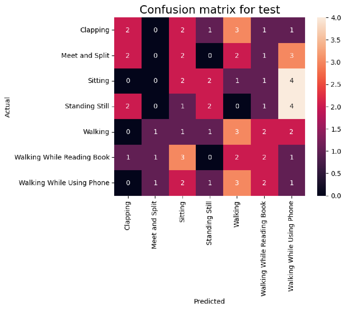
混淆矩阵
#

def get_actual_predicted_labels(dataset):
  actual = [ labels for _, labels in dataset.unbatch() ]
  predicted = model.predict(dataset)

  actual = tf.stack(actual, axis = 0)
  predicted = tf.concat(predicted, axis = 0)
  predicted = tf.argmax(predicted, axis = 1)

  return actual, predicted

def plot_confusion_matrix(actual, predicted, labels, ds_type):
  cm = tf.math.confusion_matrix(actual, predicted)
  ax = sns.heatmap(cm, annot=True, fmt='g')
  sns.set(rc={'figure.figsize': (12, 12)})
  sns.set(font_scale = 1.4)
  ax.set_title('Confusion matrix for ' + ds_type)
  ax.set_xlabel('Predicted')
  ax.set_ylabel('Actual')
  plt.xticks(rotation = 90)
  plt.yticks(rotation = 0)
  ax.xaxis.set_ticklabels(labels)
  ax.yaxis.set_ticklabels(labels)

labels = list(fg.class_ids_for_name.keys())
actual, predicted = get_actual_predicted_labels(test_ds)
plot_confusion_matrix(actual, predicted, labels, 'test')

精确率与召回率
#

def calculate_classification_metrics(actual, predicted, labels):
  cm = tf.math.confusion_matrix(actual, predicted)
  tp = np.diag(cm)
  precision = dict()
  recall = dict()
  for i in range(len(labels)):
    col = cm[:, i]
    fp = np.sum(col) - tp[i]
    row = cm[i, :]
    fn = np.sum(row) - tp[i]

    precision[labels[i]] = tp[i] / (tp[i] + fp)
    recall[labels[i]] = tp[i] / (tp[i] + fn)
  return precision, recall

precision, recall = calculate_classification_metrics(actual, predicted, labels)

精确率：预测为该类中实际正确的比例
召回率：实际为该类中被正确预测的比例

九、预览测试
#

从测试集取一个 batch，对每个视频预测类别并可视化帧序列。

def preview_test():
  ds = test_ds.take(1)
  for batch in ds:
    prediction = model.predict(batch[0])
    videos, labels = batch
    for i in range(len(labels)):
      images = videos[i]
      print(classes[np.argmax(prediction[i])])
      return to_gif(images)

preview_test()

1/1 [==============================] - 0s 84ms/step
Walking

十、总结
#

本教程实现了一个完整的视频行为识别系统，关键技术点回顾：

方面	技术方案
帧采样	跳帧采样（step=15），随机起始位置
帧标准化	resize_with_pad 统一到 224×224，float32
数据管道	tf.data + cache + shuffle + prefetch + batch
卷积核	Conv2Plus1D 分解（空间 + 时间），参数减少 55%
残差连接	跳跃连接 + LayerNorm + Project 维度对齐
空间下采样	ResizeVideo（einops 重排后 Resizing）
优化器	Adam（lr=0.0001）
损失函数	SparseCategoricalCrossentropy
评估指标	准确率、混淆矩阵、精确率、召回率

这种 (2+1)D 卷积架构平衡了计算效率和表达能力，是视频理解任务中非常实用的基线方案。完整的代码兼容 UCF-101、HMDB-51 等标准视频行为数据集，只需调整数据集路径即可迁移。

1. 环境准备 #

1.1 检查 GPU #

1.2 安装依赖 #

1.3 导入库 #

2. 数据集下载与探索 #

2.1 下载视频数据集 #

2.2 列出 ZIP 内的文件 #

2.3 提取类别名称 #

2.4 统计各类别样本量 #

3. 数据划分与下载 #

3.1 类别子集选择 #

3.2 从 ZIP 下载文件 #

3.3 数据划分函数 #

3.4 执行划分与下载 #

3.5 验证数据分布 #

四、视频帧提取与预处理 #

单帧格式化 #

从视频文件中提取帧序列 #

帧生成器类 #

五、数据管道构建 #

六、(2+1)D 卷积模型 #

Conv2Plus1D：分解 3D 卷积 #

残差模块 #

视频下采样 #

完整模型结构 #

七、模型编译与训练 #

八、模型评估 #

混淆矩阵 #

精确率与召回率 #

九、预览测试 #

十、总结 #